We show that deep reinforcement learning is successful at optimizing SQL joins, a problem studied for decades in the database community. Further, on large joins, we show that this technique executes up to 10x faster than classical dynamic programs and 10,000x faster than exhaustive enumeration. This blog post introduces the problem and summarizes our key technique; details can be found in our latest preprint, Learning to Optimize Join Queries With Deep Reinforcement Learning.
SQL query optimization has been studied in the database community for almost 40 years, dating all the way back from System R’s classical dynamic programming approach. Central to query optimization is the problem of join ordering. Despite the problem’s rich history, there is still a continuous stream of research projects that aim to better understand the performance of join optimizers in realistic multi-join queries, or to tackle the very large join queries that are ubiquitous in enterprise-scale “data lakes”.
In our latest preprint, we show that deep reinforcement learning (deep RL) provides a new angle of attack at this decade-old challenge. We formulate the join ordering problem as a Markov Decision Process (MDP), and we build an optimizer that uses a Deep Q-Network (DQN) to efficiently order joins. We evaluate our approach on the Join Order Benchmark (a recently proposed workload to specifically stress test join optimization). Using only a moderate amount of training data, our deep RL-based optimizer can achieve plan costs within 2x of the optimal solution on all cost models that we considered, and it improves on the next best heuristic by up to 3x — all at a planning latency that is up to 10x faster than dynamic programs and 10,000x faster than exhaustive enumeration.
Background: Join ordering
Why is reinforcement learning a promising approach for join ordering? To answer this question, let’s first recap the traditional dynamic programming (DP) approach.
Assume a database consisting of three tables, Employees, Salaries, and Taxes. Here’s a query that calculates “the total tax owned by all Manager 1 employees”:
SELECT SUM(S.salary * T.rate)
FROM Employees as E, Salaries as S, Taxes as T
WHERE E.position = S.position AND
T.country = S.country AND
E.position = ‘Manager 1’
This query performs a three-relation join. In the following example, we use J(R) to denote the cost of accessing a base relation R, and J(T1,T2) the cost of joining T1 and T2. This is the cost model that we assume a DBMS has built in (e.g., a deterministic scoring function). For simplicity, we assume one access method, one join method, and a symmetric join cost (i.e., J(T1, T2) = J(T2, T1)).
The classical “left-deep” DP approach first calculates the cost of optimally accessing the three base relations; the results are put in a table:
| Remaining Relations | Joined Relations | Best |
| {E, S} | {T} | J(T), i.e., scan cost of T |
| {E, T} | {S} | J(S) |
| {T, S} | {E} | J(E) |
Then, it builds off of this information and enumerates all 2-relations. For instance, when calculating the best cost to join {E,S}, it looks up the the relevant, previously computed results as follows:
Best({E, S}) = Best({E}) + Best({S}) + J({E}, S)
which results in the following row to be added into the table:
| Remaining Relations | Joined Relations | Best |
| {T} | {E, S} | Best({E}) + Best({S}) + J({E}, S) |
The algorithm proceeds through other 2-relation sets, and eventually to the final best cost for joining all three tables. This entails taking the minimum over all possible “left-deep” combinations of 2-relations and a base relation:
| Remaining Relations | Joined Relations | Best |
| {} | {E, S, T} | minimum { Best({E,T}) + J(S) + J({E,T}, S), Best({E,S}) + J(T) + J({E,S}, T), Best({T,S}) + J(E) + J({T,S}, E) } |
The dynamic program is now complete. Note that J’s second operand (relation on the right) is always a base relation, whereas the left could be an intermediate join result (hence the name “left-deep”). This algorithm has a space and time complexity exponential in the number of relations, which is why it’s often used only for queries with ~10-15 relations.
Join Ordering via Reinforcement Learning
The main insight of our work is the following: instead of solving the join ordering problem using dynamic programming as shown above, we formulate the problem as a Markov Decision Process (MDP) and solve it using reinforcement learning (RL), a general stochastic optimizer for MDPs.
First, we formulate join ordering as an MDP:
- States, G: the remaining relations to be joined.
- Actions, c: a valid join out of the remaining relations.
- Next states, G’: naturally, this is the old “remaining relations” set with two relations removed and their resultant join added.
- Reward, J: estimated cost of the new join.
Or (G, c, G’, J) for short.
We apply Q-learning, a popular RL technique, to solve the join-ordering MDP. Let us define the Q-function, Q(G, c), which, intuitively, describes the long-term cost of each join: the cumulative cost if we act optimally for all subsequent joins after the current join decision.
Q(G, c) = J(c) + \min_{c’} Q(G’, c’)
Notice how if we have access to the true Q-function, we can order joins in a greedy fashion:
Algorithm 1
(1) Start with the initial query graph,
(2) Find the join with the lowest Q(G, c),
(3) Update the query graph and repeat.
As it turns out, Bellman’s Principle of Optimality tells us that this algorithm is provably optimal. What’s fascinating about this algorithm is that it has a computational complexity of O(n^3), which, while still high, is much lower than the exponential runtime complexity of exact dynamic programming.
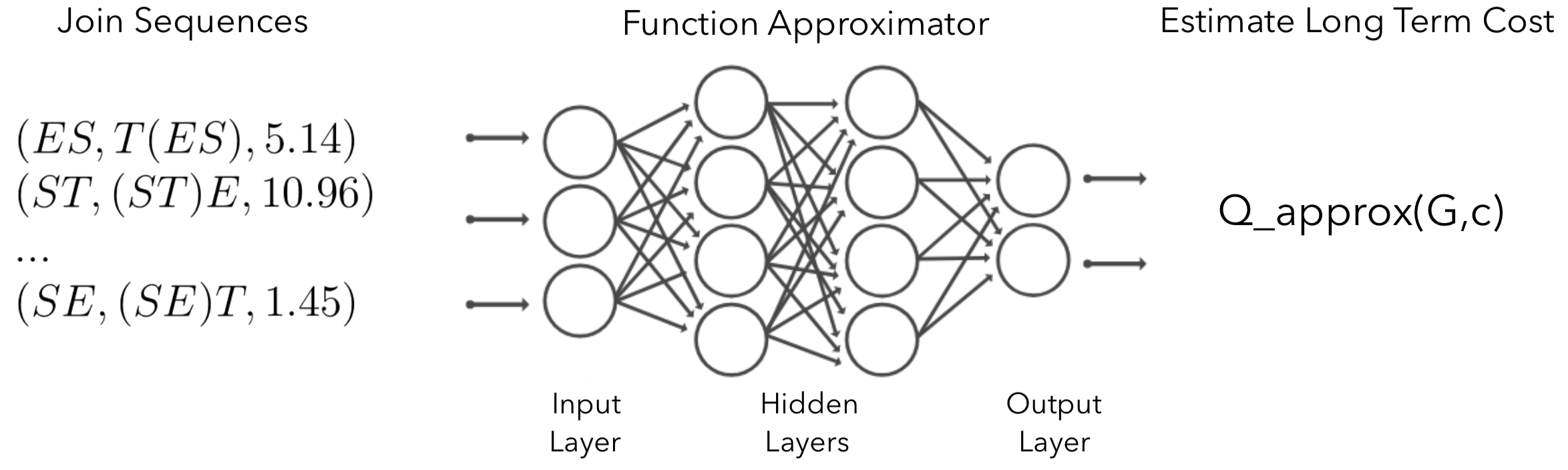 Figure 1: Using a neural network to approximate the Q-function. Intuitively, the output means “If we make a join c on the current query graph G, how much does it minimize the cost of the long-term join plan?”
Of course, in reality we don’t have access to the true Q-function and would need to approximate it. To do so we use a neural network (NN). When an NN is used to learn the Q-function, the technique is called Deep Q-network (DQN). This is the same technique used to successfully learn to play Atari games with expert-level capability. To summarize, our goal is to train a neural net that takes in (G, c) and outputs an estimated Q(G,c); see Figure 1.
Meet DQ, the Deep Reinforcement Learning Optimizer
Enter DQ, our deep RL-based optimizer.
Data collection. To learn the Q-function we first need to observe past execution data. DQ can accept a list of (G, c, G’, J) from any underlying optimizer. For instance, we can run a classical left-deep dynamic program (as shown in the Background section) and calculate a list of “join trajectories” from the DP table. A tuple out of a complete trajectory could look something like (G, c, G’, J) = ({E, S, T}, join(S, T), {E, ST}, 110), which represents the step of starting with the initial query graph (state) and joining S and T together (action).
Although we’ve described J to be the estimated cost of a join, we can use the actual runtime too if data is collected from a real database execution.
Featurization of states and actions. Since we are using a neural net to represent Q(G, c), we need to feed states G and actions c into the network as fixed-length feature vectors. DQ’s featurization scheme is very simple: we use 1-hot vectors to encode (1) the set of all attributes present in the query graph, out of all attributes in the schema, (2) the participating attributes from left side of the join, and (3) those from right side of the join. This is pictorially depicted in Figure 2.
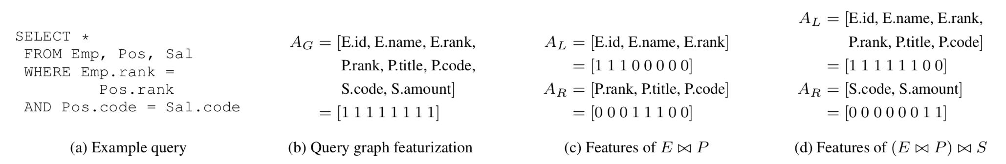
Figure 2: A query and its corresponding featurizations. We assume a database of Employees, Positions, and Salaries. A partial join and a full join are shown. The final feature vector of (G,c) is the concatenation of A_G (attributes of query graph), A_L (attributes of the left side), and A_R (attributes of the right side).
Although this scheme is extremely straightforward, we’ve found it to be sufficiently expressive. Note that our scheme (and the learned network) assumes a fixed database since it needs to know the exact set of attributes/tables.
Neural network training & planning. By default, DQ uses a simple 2-layer fully connected network. Training is done with standard stochastic gradient descent. Once trained, DQ accepts a SQL query in plain text, parses it into an abstract syntax tree form, featurizes the tree, and invokes the neural network whenever a candidate join is scored (i.e., the neural net is invoked in step 2 of Algorithm 1). Lastly, DQ can be periodically re-tuned using the feedback from real execution.
Evaluation
To evaluate DQ, we use the recently published Join Order Benchmark (JOB). The database consists of 21 tables from IMDB. There are 33 query templates and a total of 113 queries. The join sizes in the queries range from 5 to 15 relations. Here, DQ collects training data from exhaustive enumeration when the number of relations to join is no larger than 10, and from a greedy algorithm for the additional relations.
Comparison. We compare against several heuristic optimizers (QuickPick; KBZ) as well as classical dynamic programs (left-deep; right-deep; zig-zag). The plans produced by each optimizer are scored and compared to the optimal plans, which we obtain via exhaustive enumeration.
Cost models. With new hardware innovations (e.g., NVRAM) and a move towards serverless RDBMS architectures (e.g., Amazon Aurora Serverless), we expect to see a multitude of new query cost models that capture distinct hardware characteristics. To show a learning-based optimizer can adapt to different environments unlike fixed heuristics, we design 3 cost models:
- Cost Model 1 (Index Mostly): models a main-memory database and encourages index joins.
- Cost Model 2 (Hybrid Hash): considers only hash joins and nested loop joins with a memory budget.
- Cost Model 3 (Hash Reuse): accounts for the reuse of already-built hash tables.
As we go from CM1 to CM3, the costs are designed to have more non-linearity, posing challenges to static strategies.
We do 4-fold cross validation to ensure DQ is only evaluated on queries not seen in the training workload (in each case, we train on 80 queries and test on 33). We calculate the mean sub-optimality of the queries, i.e., “cost(plan from each algorithm) / cost(plan from optimal plan)”, so lower is better. For instance, on Cost Model 1, DQ is on average 1.32x away from optimal plans. The results are shown in Figure 3.
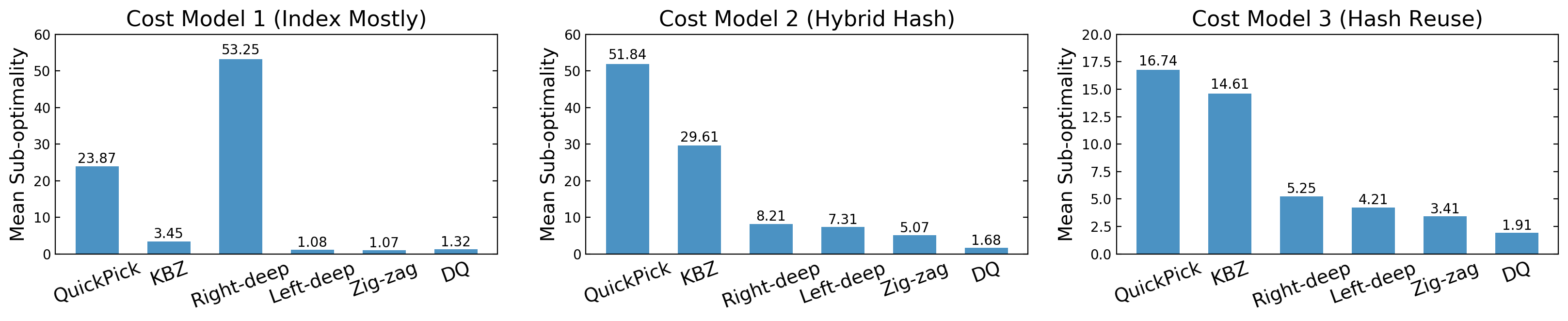 Figure 3: Mean plan sub-optimality (w.r.t. exhaustive enumeration) under different cost models.
Across all cost models, DQ is competitive with the optimal solution without a priori knowledge of the index structure. This is not true for fixed dynamic programs: for instance, left-deep produces good plans in CM1 (encourages index joins), but struggles in CM2 and CM3. Likewise, right-deep plans are uncompetitive in CM1 but if CM2 or CM3 are used, the right-deep plans suddenly become not so bad. The takeaway is that a learning-based optimizer are more robust than hand-designed algorithms and can adapt to changes in workload, data, or cost models.
Furthermore, we show that DQ produces good plans at a much faster speed than classical dynamic programs (Figure 4).
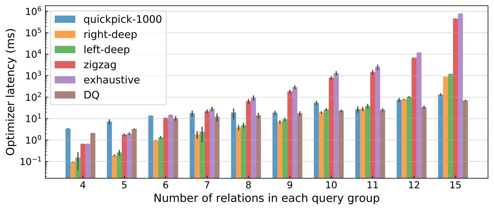
Figure 4: Optimizer latency on all 113 JOB queries (log-scaled), grouped by the number of relations in the query. Error bars represent ± standard deviation around the mean; a total of 5 trials were run.
In the large-join regime, DQ achieves drastic speedups: for the largest joins DQ wins by up to 10,000x compared to exhaustive enumeration, over 1,000x faster than zig-zag, and more than 10x faster than left/right-deep enumeration. The gain mostly comes from the abundant batching opportunities in neural nets — for all candidate joins of an iteration, DQ batches them and invokes the NN once on the entire batch. We believe this is a profound performance argument for such a learned optimizer: it would have an even more unfair advantage when applied to larger queries or executed on specialized accelerators (e.g., GPUs, TPUs).
Summary
In this work, we argue that joining ordering is a natural problem amenable to deep RL. Instead of fixed heuristics, deep RL uses a data-driven approach to tailor the query plan search to a specific dataset, query workload, and observed join costs. To select a query plan, DQ uses a neural network that encodes the compressed versions of the classical dynamic programming tables observed at training time.
DQ touches only the tip of the iceberg. In the database and systems communities, intensifying debate has revolved around putting more learning, or in other words, data adaptivity, into existing systems. We hope our work represents the first step in enabling more intelligent query optimizers. For more details, please refer to our Arxiv preprint.